This step-by-step tutorial uses the Intro-to-HCA-data-on-Terra workspace to import, access, and analyze Human Cell Atlas (HCA) data with community-supported single-cell tools like Bioconductor, Cumulus, Pegasus, Scanpy, and Seurat.
Human Cell Atlas Overview
The Human Cell Atlas (HCA) project is a global initiative aiming to create comprehensive reference maps of all human cells. Researchers can share and find HCA single-cell data through the HCA's Data Coordination Platform (DCP), the project's data contribution, access, and analysis service.
The DCP maintains the HCA Data Portal where you can browse HCA projects and find data of interest (see the portal's guides to get started).
The Data Portal hosts multiple data types, including metadata files, raw sequencing files (FASTQs), contributor-generated matrices that contain cell by gene count data from the project contributors, and preprocessed data (BAMs and cell by gene count matrices in Loom format) generated using standardized pipelines approved by HCA Analysis Working Group.
This tutorial provides step-by-step instructions for finding HCA data, importing it into a Terra workspace, and analyzing it with workflows and Jupyter Notebooks. Although this tutorial uses an example DCP-generated project count matrix (read more in the Data Portal's matrix overview), you can use the import steps for all data types.
Step 1: Clone the Intro-to-HCA-data-on-Terra workspace
Before you begin, create your own editable copy (clone) of the Intro-to-HCA-data-on-Terra workspace by following the instructions in How to clone your own workspace. For this tutorial, you do not need an authorization domain.
After cloning, take a few minutes to explore the workspace.
- Look at the Data page and explore the participant data table. This data table is preloaded with example data.
- When you import any HCA data to Terra (as you'll do in the next section), the participant data table is created automatically. The name "participant" was chosen by the DCP team, but you can (re)name Terra data tables as you like.
- Data tables do not actually contain raw data, but include links to the data in cloud storage, such as a Google bucket.
- Next, select the Workflows page which contains the Cumulus workflow for large-scale single-cell analysis- we'll run this workflow in a later section.
- Lastly, glance at the Notebooks page; it has notebooks for single-cell analysis using four community-supported tools: Bioconductor, Pegasus, Scanpy, and Seurat.
Step 2: Import HCA data from the HCA Data Portal
HCA data is imported from the DCP's Data Portal. For this tutorial, we'll show you how to import DCP-generated cell by gene matrices (Loom file format) for the 10x single-cell RNA sequencing project SingleCellLiverLandscape.
We already imported this data for you in the Intro-to-HCA-data-on_Terra workspace, but you can either repeat these steps or use them to find and import more data files.
Step-by-step instructions
2.1. Navigate to the Data Portal's Data Browser.
At the top of the page, you'll notice a faceted search box that allows you to filter HCA data by project title, donor information, tissue types, disease states, and more. At the bottom of the page, you'll see a list of HCA projects.
2.2. In the Search all filters field of the faceted search box, start typing the project's short name ("SingleCellLiverLandscape...").
Screenshot of SingleCellLiverLandscape in dropdown
A list of project titles that match the search terms appears in the search box. Select the tutorial project (SingleCellLiverLandscape).
2.3. In the project list, select the checkbox (to the left of the project name).
Screenshot of Export Selected Data button
2.4. Choose the Export Selected Data button.
2.5. Under the Analyze in Terra section, select Start.
2.6. Select the species (only "Homo sapiens" option available for this project).
2.7. Select the files to export; for cell by gene count matrices, choose "loom".
Screenshot of file types
You could also choose the raw FASTQ files, the standardized BAM files (one for each library preparation), or additional file types provided by the project contributor. The types of contributor-generated files will vary across projects (some will have CSV, h5ad, etc.).
2.8. Select Request Link.
It takes a few seconds to prepare the export.
2.9. When the export is ready, click the link.
Screenshot of export link to click
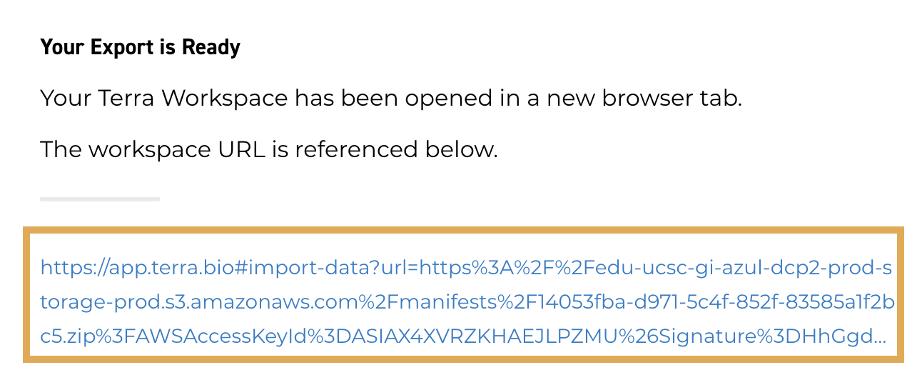
You'll be redirected to the Terra platform and prompted to select a destination workspace.
2.10. Choose Start with an existing workspace.
2.11. Type the name of your cloned workspace or choose it from the drop-down menu.
Screenshot of existing workspace dropdown
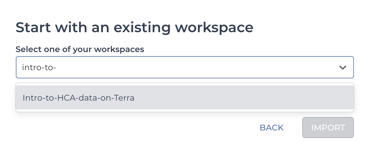
2.12. Select Import.
2.13. Refresh the workspace Data page to view your data.
What to expect
Terra automatically generates a participant data table for the selected data. If you (re)import the example matrices for this tutorial's example, Terra overwrites the existing data table. If you import additional data files, Terra adds them to the existing participant data table.
2.14. Explore the columns of the participant data table.
The first column contains a participant ID, which is a unique identifier (UUID) for the analysis bundle. This table has multiple UUIDs for different metadata, but if you scroll right, you'll see plenty of human-readable metadata as well.
Screenshot of participant table
What to expect
This project has multiple donors, each with their own 10x library preparation and analysis output. The project also has a combined analysis for all 5 donors (a project matrix).
Each row of the table represents these different project analysis files. The first row contains the metadata and file links for the combined project analysis (all 5 donors); the subsequent rows contain information/files for each individual donor (one donor per row).
The subsequent table columns contain information about the individual data files as well as metadata relating to the project's donors, organs, developmental stages, disease states, and data processing criteria.
Information pertaining to this tutorial's example count matrix files can be found in columns with the "_loom_" prefix. As you scroll through these columns, remember, the data table does not contain the actual loom files but rather links to the loom files in their cloud location (a Google bucket in this case). To see this, go to the __loom__file_drs_uri column and click on one of the links. It will launch a File Details window.
Screenshot of file details popup
In the File Details, you can view the file in its Google bucket location, download the file or use command-line tools to access the file.
What are DRS URIs?
The cloud location links for each matrix file are in the form of a DRS (Data Repository Service) URI listed in the __loom__file_drs_uri column. DRS URIs are cloud-agnostic identifiers that allow Terra to pull files from diverse repositories (Amazon Web Services, Azure, Google bucket, etc.). Read more about the identifiers in the overview Data Access with the GA4GH Data Repository Service (DRS).
Step 3: Filter, cluster and normalize a 10x count matrix using Cumulus
Cumulus is a cloud-based analysis workflow for large-scale single-cell and single-nucleus RNA-seq data (Li et al. 2020). The workflow takes in a raw count matrix and performs filtering, normalization, and clustering.
The Cumulus workflow in the Intro-to-HCA-data-on-Terra workspace is already set up to read the tutorial's project matrix (sc-landscape-human-liver-10XV2.loom) which is listed in the workspace participant data table. This project matrix contains raw counts for 10x liver data processed with the Optimus pipeline.
All Data Portal project matrices contain counts from library preparations (can be multiple donors) of the same species, organ, developmental stage, and technology. They're identified by their filename which follows the format "<project-description>-<species>-<organ>-<sequencing technology>.loom".
Example filename format
sc-landscape-human-liver-10XV2.loom
To learn more about the different types of matrices, read the Data Portal's Matrix Overview.
Step-by-step instructions
3.1. Go to the participant data table on the Data page and select the checkbox left of the participant_ID.
01335551-3f19-5ce1-9b0a-5828423e9725.2021-02-02T133000.000000Z
3.2. Select the “Open with” icon.
Screenshot of Open with icon
3.3. Select Workflow.
3.4. Select the Cumulus workflow
Screenshot of Cumulus workflow
You'll be redirected to the workflow setup page.
3.5. Explore the workflow Input and Output tabs.
The workflow is set up to run Cumulus on the Loom file listed in the __loom__file_drs_uri column of the participant table.
Additionally, there are multiple Cumulus parameters set up for you which you can learn in the Cumulus overview.
3.6. Go to the workflow Inputs tab
3.7. Make sure the input_file variable is specified as the column with the Optimus loom file
What to expect
For this tutorial, the input_file attribute should be “this.__loom__file_drs_uri,” which points to the cloud location for the example project matrix.
Screenshot of input_file attribute
3.8. Change the input attribute for the output_directory variable to a Cumulus folder in your Workspace Google bucket.
What to expect
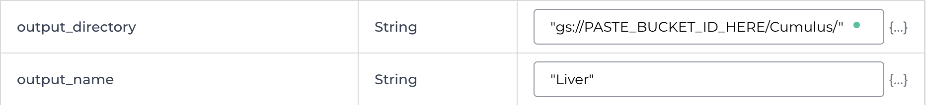
The attribute is preset to “gs://PASTE_BUCKET_ID_HERE/Cumulus/”. Just paste your Google bucket ID over the PASTE_BUCKET_ID_HERE section.
Example output_directory variable
What to use
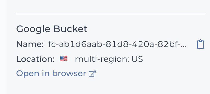
You can find the Google bucket location on the right of your workspace Dashboard.
Where to find your Google bucket ID
Attribute string example
For example, if your Google bucket ID is fc-c3efdef7-76f2-4ffb-8e29-479bf9758df9, you would use the following string for the attribute:
“gs://fc-c3efdef7-76f2-4ffb-8e29-479bf9758df9/Cumulus/”
3.9. Check the output_name attribute.
The output_name is a prefix that is used to name the output files and to name an output file folder. By default, it is set to "Liver" because this tutorial uses example liver data. You can change this value to any string that is meaningful to your selected data or you can configure this from the data table using one of the existing columns (i.e., participant_id).
3.10. Select Save.
3.11. Do not specify any output attributes in the Workflow Outputs tab.
Why this warning?
Cumulus places outputs in the directory specified on the inputs tab, which in this example write to the Files subsection of the Other Data section on the workspace Data page. Currently, Cumulus isn't configured to write outputs to a Terra data table.
3.12. Select RunAnalysis and then Launch.
What to expect
You'll be redirected to the Job History page. When the workflow successfully completes, you'll see a green checkmark and the word “Succeeded”.
Screenshot of successful submission
3.13. Go to the Data page and select Files in the Other Data section.
Screenshot of Files
3.14. Select the “Cumulus” folder and then the “Liver folder to see the outputs.
3.15. Take a look at the different file types Cumulus produces, which include differential expression files (de.xlsx), as well as visualization files. You can check the Cumulus documentation for a full description.
Screenshot of liver files generated by Cumulus
How to find output files
Some of the outputs have a “.scp” suffix; these are outputs that are compatible with Single Cell Portal, a platform allowing you to visualize cell clusters identified by Cumulus.
Step 4. Explore HCA data using Jupyter Notebooks
You can process and visualize single-cell data using common community-supported tools that can run in a Jupyter Notebook. The Intro-to-HCA-data-on-Terra workspace has four notebooks with example code to help you get started with single-cell analysis in R or Python environments.
Each tutorial is designed to help you
- Import a project matrix into your Cloud Environment
- Subset the project matrix to a demo size for the tutorial
- Filter cells based on quality control metrics
- Normalize cell counts
- Cluster and visualize cells
- Test clusters for differential gene expression
Bioconductor notebook
The Bioconductor notebook (R environment) uses a modified version of the "Orchestrating single-cell analysis with Bioconductor" (Amezquita et al., 2020) tutorial to analyze the project count matrix for SingleCellLiverLandscape. It converts the Loom matrix into a SingleCellExperiment object that can be used with Bioconductor tools.
Convert Loom to Seurat notebook
This tutorial (R environment) uses the sceasy package to convert the SingleCellLiverLandscape project Loom matrix to a Seurat object that can be used with a modified version of Seurat's Guided Clustering Tutorial in the Seurat notebook (described below).
Pegasus notebook
Pegasus is a Python package for single-cell analysis and also part of Cumulus. The Pegasus notebook uses a modified version of the Pegasus Tutorial to analyze the project count matrix for SingleCellLiverLandscape. It reads the Loom files using a custom function, read_input(), and then performs downstream filtering, normalizing, clustering, and differential expression analysis.
Scanpy notebook
The Scanpy notebook (Python environment) uses a modified version of the "Preprocessing and clustering 3k PBMCs" tutorial to convert the SingleCellLiverLandscape project Loom matrix into an AnnData object that can be analyzed with Scanpy.
Seurat notebook
The Seurat notebook (R environment) performs single-cell analysis (filtering, normalizing, clustering, and visualization) of the SingleCellLiverLandscape project matrix, which has been preconverted to a Seurat object using the "Convert_Loom_to_Seurat" notebook. This tutorial is a modified version of Seurat's Guided Clustering Tutorial.
Step-by-step instructions
4.1. Before starting, use the table below to identify the Cloud Environment configuration for the tool you want to try.
| Notebook | Application Configuration |
| Bioconductor | R/Bioconductor |
| Convert_Loom_to_Seurat | R/Bioconductor |
| Pegasus | Pegasus (community-maintained environment) |
| Scanpy | R/Bioconductor |
| Seurat | R/Bioconductor |
4.2. Select the Environment Configuration widget in the right corner of the workspace.
4.3. Under Jupyter, select the Environment Settings.
4.4. At the bottom of the dialogue box, select Create custom environment.
4.5. Based on Step 1 above, select the appropriate software option from the Application configuration drop-down.
For example, if you're using the Bioconductor notebook, select the R/Bioconductor configuration.
4.6. For the Cloud Compute Profile, use 4 CPUs.
4.7. Select Create to start the Cloud Environment VM.
4.8. From the Analyses page, select the tutorial notebook you want to use.
4.9. Click on the Edit button (at the top) and follow the notebook instructions to analyze and visualize single-cell data.
Congratulations! You’ve completed the Intro-to-HCA-data-in-Terra Tutorial. To learn more about how to use Terra or the different tools showcased in this tutorial, see the Resources section below.
Learn more with Terra and single-cell resources
Terra support documentation, videos, and workspaces
Get started on Terra with Terra support materials. These resources teach you the basics of creating and using data tables, importing and running workflows, and using Jupyter Notebooks.
Terra Support
- Terra support documentation
- Terra support videos
- Terra Data Tables Quickstart Featured Workspace
- Terra Workflows Quickstart Featured Workspace
- Terra Notebooks Quickstart Featured Workspace
Single-cell resources
- HCA Data Coordination Platform and Data Portal for data contribution and guides to using HCA data
- Optimus Featured Workspace in Terra for preprocessing 10x single-cell data
- Cumulus Featured Workspace in Terra for filtering, normalizing, and clustering single-cell data
- Bioconductor for single-cell analysis tools in R
- Pegasus for single-cell analysis in python
- Scanpy for single-cell analysis in python
- Seurat for single-cell analysis in R
Next steps
Check the workspace changelog for the latest updates to the workspace.
Want to add your tool to the workspace?
Add your comments and feedback using the Terra Featured Workspace community forum.
References
- Amezquita, R.A., Lun, A.T.L., Becht, E. et al. Orchestrating single-cell analysis with Bioconductor. Nat Methods 17, 137–145 (2020). https://doi.org/10.1038/s41592-019-0654-x
- Butler, A., Hoffman, P., Smibert, P. et al. Integrating single-cell transcriptomic data across different conditions, technologies, and species. Nat Biotechnol 36, 411–420 (2018). https://doi.org/10.1038/nbt.4096.
-
Dissecting the human liver cellular landscape by single cell RNA-seq reveals novel intrahepatic monocyte/ macrophage populations
- Li, B., Gould, J., Yang, Y. et al. Cumulus provides cloud-based data analysis for large-scale single-cell and single-nucleus RNA-seq. Nat Methods 17, 793–798 (2020). https://doi.org/10.1038/s41592-020-0905-x
- MacParland, Sonya A et al. “Single cell RNA sequencing of human liver reveals distinct intrahepatic macrophage populations.” Nature communications vol. 9,1 4383. 22 Oct. 2018, doi:10.1038/s41467-018-06318-7
- Stuart T, Butler A, Hoffman P, Hafemeister C, Papalexi E, Mauck WM 3rd, Hao Y, Stoeckius M, Smibert P, Satija R. Comprehensive Integration of Single-Cell Data. Cell. 2019 Jun 13;177(7):1888-1902.e21. doi: 10.1016/j.cell.2019.05.031.