Hands-on practice setting up and running a Jupyter notebook in a cloud environment VM. This workspace is the last of three tutorials that feature a mock study of the correlation between heights and grades for a cohort of 7th, 8th, and 9th graders. In part 3 of the Quickstart, you'll run an interactive Jupyter analysis to import and compare processed data from the workflows tutorial for a small cohort and then the full dataset.
Importing and plotting data generated in a workflow analysis is the last step to discover if there is a correlation between student height and grades.
Prerequisite
You should have already completed the Data Tables and Workflows tutorials. You will work in your copy of the Quickstart workspace to get hands-on to learn about analyzing data in a notebook.
Notebooks tutorial learning objectives
In this tutorial, you'll plot height versus average GPA for students in the study and answer the study question you're exploring: does a student's height affect their grade point average?
Part 3 of the Quickstart is intended to help you become familiar with interactive analysis on Terra, a second mode of analysis you can do in your Terra workspace. Although the tutorial focus is a Jupyter analysis, many of the steps for setting up a cloud environment are similar when running Galaxy or RStudio.
After working through the Quickstart exercises, you will know how to
- Set up a Jupyter Cloud Environment in Terra
- Open and run a Jupyter Notebook
- Import primary data from a data table into a notebook for analysis
- Visualize study data and compare results from small and large datasets
Estimated Time and cost requirements You should be able to complete part 3 of the Quickstart in half an hour or less. Running the tutorial will cost less than $0.25 (Google Cloud data storage and VM costs).
Additional requirements
You should have completed part 1 (data tables) and part 2 (workflows) of the Quickstart in your own Terra on GPC Quickstart workspace.
Three steps to complete the notebook Quickstart.
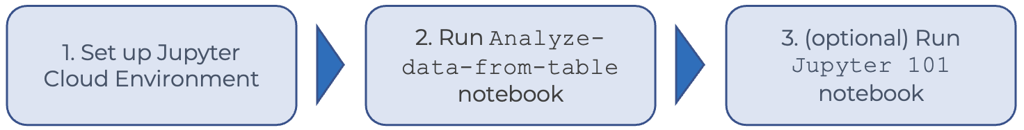
Part 1: Set up a Jupyter Cloud Environment
Part 2: Import data and run the Analyze-data-from-table notebook
Part 3: (optional) Run the Jupyter 101 notebook
New to Jupyter notebooks?While it is possible to set up the Jupyter cloud environment and run a notebook without any prior knowledge of Jupyter Notebooks, it may be useful to read the Jupyter 101 notebook to learn the basics
- How to use a notebook
- How to install packages
- How to import data
- Why notebooks are useful in biomedical research
Notebooks Quickstart - step-by-step guide and video
Work in your own copy of the Quickstart workspace
Now that you've gotten familiar with the mock study data and done some initial processing of the raw data, you're ready to view the results. You'll get hands-on practice with interactive analysis in Terra running a notebook to plot the heights versus grades for the subset and the full dataset of middle school students.
Video walkthrough instructions
1. Set up Jupyter Cloud Environment
The interactive Jupyter app runs in a fully customizable Cloud Environment VM in Terra. You will need to set up and launch the Jupyter Cloud Environment the first time you run a notebook in the workspace.
1.1. Start in the Analyses tab of your workspace.
1.2. Click the cloud icon in the right sidebar.
1.3. In the Cloud Environment Details pane, click the gear icon (Environment settings) under the Jupyter logo. This will surface the Jupyter Cloud Environment default pane (below).
1.4. Click the Create button to start a Jupyter Cloud Environment with the default settings.
What to expect
Once you click Create, it will take a few minutes for the Jupyter Cloud Environment to start. During this time, Terra is requesting and setting up the Google resources to run the notebook.
You can also get to the (Jupyter) Cloud Environment pane by clicking the notebook name.
Note on billing when running a notebook
- Billing begins when your Cloud Environment is created and continues until you pause or delete it, regardless of whether the VM is running any computations.
- Every time you open a notebook, a new Jupyter kernel is created.
- If you have multiple notebooks open and running in a single workspace, they will all consume resources (memory and CPU) on the same Cloud Environment.
Note on billing for Detachable Persistent Disks
- When you delete your Cloud Environment, you can choose to keep your Detachable Persistent Disk. If you do, you will incur a charge of $2.00/month (50 GB disk).
Note that your workspace Cloud Environment is yours and yours aloneNo one else - even collaborators in the same workspace - can view or access data generated in a notebook and stored in your Cloud Environment persistent disk. The reason for this is security. We store your Google credentials on the Google VM, which cannot be shared with other users.
2. Run the notebook Analyze-data-from-table
Once your Cloud Environment is running, you'll see a green dot just below the Jupyter logo in the right sidebar. You can now dive into this tutorial notebook to answer the burning question of whether and how height influences GPA (for a cohort of middle-schoolers)
Step-by-step instructions
2.1. Click on “Analyze-data-from-table” in the Analyses tab of your clone of the Quickstart workspace.
2.2. Click on the Open button at the top of the Preview so you can edit and run the code in the notebook.
To learn more about "Playground" mode, see this article
2.3. Skim the read-only view for an overview of what's in the notebook.
2.4. Run the first code cell: click in the cell and then click Run from the menu at the top to execute the code in that cell. Note - you can also use the shortcut “shift” + “return” to run a cell.
2.5. Wait for the * at the left of the cell to turn into a number, i.e. ['*'] --> [4], which indicates that the code in the cell has executed successfully.
2.6. Click in the next cell and then click Run to execute the code in the next cell. Wait for execution to complete and review the results,
2.7. Repeat step 6 until you've executed the code in all cells from the notebook. Make sure to read the documentation to understand the point of each code block. Note that good documentation means you don't have to be able to code to run a notebook analysis!
2.8. When you've run all the code cells, pause the Jupyter cloud environment by clicking the Jupyter logo in the sidebar and clicking on the pause icon.
2.9. Close the notebook by clicking the green x in the top right.
Thought Questions
Looking at the graph of the eight-student subset, what seems to be the relationship between height and cumulative GPA in the subset cohort? Does this relationship seem reasonable?
-
It seems from this plot that GPA increases linearly with height (taller students get better grades).
This seems unlikely, but it is a sample set of only eight students...
How does your graph change based on plotting the full dataset? Is this graph more expected? What did this exercise show you about the importance of sample size in data?
-
The larger sample size gives a clearer picture of the relationship (or lack thereof) between height and GPA.
This simple analysis example shoes the basic steps to run a Notebook analysis in Terra (GCP) and also demonstrates the importance of large sample sizes to boost the confidence in your study results.
🎉 🎉 Congratulations! You've finished the three Terra on GCP Quickstart tutorials 🎉 🎉
3. (optional) Explore the Jupyter 101 tutorial notebook
If you aren't familiar with Jupyter notebooks, you can try out this primer at your own pace.
Dive into this tutorial notebook to learn more about
- Why notebooks are used in biomedical research
- The relationship between the notebook and the workspace
- Jupyter Notebook basics: how to use a notebook, install packages, and import modules
- Common libraries in data analysis and popular tutorial notebooks